Statistical Learning

Suppose that we observe a quantitative response $Y$ and p different predictors, $X_1, X_2, . . . , X_p$. We assume that there is some relationship between $Y$ and $X = (X_1,X_2,...,X_p)$, which can be written in the very general form

$Y =f(X)+\varepsilon$

Here f is some fixed but unknown function of $X_1, . . . , X_p$, and $\varepsilon$ is a random error term, which is independent of $X$ and has mean zero.

Why do we need to estimate $f$

Prediction

In many situations, a set of inputs $X$ are readily available, but the output $Y$ cannot be easily obtained. In this setting, since the error term averages to zero, we can predict $Y$ using

$\hat{Y} = \hat{f}(X)$

where $\hat{f}$ represents our estimate for $f$, and $\hat{Y}$ represents the resulting prediction for $Y$.

The accuracy of $\hat{Y}$ as a prediction for $Y$ depends on two quantities, which we will call the reducible error and the irreducible error. In general, $\hat{f}$ will not be a perfect estimate for $f$, and this inaccuracy will introduce some error. This error is reducible because we can potentially improve the accuracy of $\hat{f}$ by using the most appropriate statistical learning technique to estimate $f$.

Since $Y$ is a function of $\varepsilon$, Even if we estimate $f$ very well we cannot reduce this error (Irreducible error).

Why is there an irreducible error?

This is because there can be unmeasurable variations and dependencies

$E(Y-\hat{Y})^2 = E[f(X) + \varepsilon - \hat{f}(X)]^2 = [f(X)-\hat{f}(X)]^2 + Var(\varepsilon)$

Inference

One may be interested in the following questions

1. Which predictors are associated with the response?
2. What is the relationship between predictor and response?
3. Can the relationship be summarized as linear or is it more complicated?

How to estimate $f$?

Parametric methods

We make some assumptions about $f$

$f(X) = \beta_0 +\beta_1X_1 +\beta_2X_2 +...+\beta_pX_p$

Then finding $f$ boils down to finding parameters $\beta$

The potential disadvantage of parametric method is if the actual $f$ is too far from our assumption, then our estimations will be poor. This can be reduced by using more flexible models which may cause overfitting

Non-parametric methods

It estimates $f$ by using near by data points. Since we are not fixing $f$, This is the advantage over parametric methods

Disadvantage in this method is it requires a large number of data points to get accurate estimate of $f$

Supervised vs Unsupervised learning

Supervised learning is where you have input variables $x$ and an output variable $Y$ and you use an algorithm to learn the mapping function from the input to the output.

Ex: Regression, Classification

Unsupervised learning is where you only have input data $X$ and no corresponding output variables.

Ex: Clustering

Assessing Model accuracy

Measuring the quality of fit

Mean squared error $MSE = 1/n(\textstyle\sum_{i=1}^n (y_i - \hat{f}(x_i))^2)$

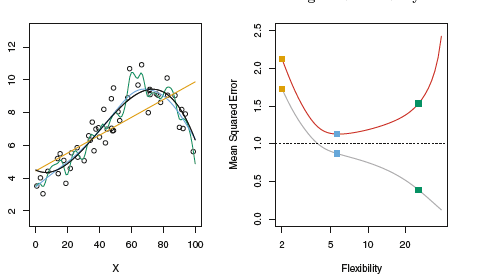
The red color in right side of the figure is test MSE and other one is training MSE

As the flexibility increases beyond the limit training error decreases but the test error increases, This is called overfitting

Bias-Variance tradeoff

Given $x_0, y_0$ as test data

$E(y_0-\hat{f}(x_0))^2 = E[y_0^2 + \hat{f}^2(x_0) - 2y_0\hat{f}(x_0)]$ $\Rightarrow E[y_0^2] + E[\hat{f}^2(x_0)] - E[2y_0\hat{f}(x_0)]$ $\Rightarrow Var(y_0) + E[y_0]^2 + Var(\hat{f}(x_0)) + E[\hat{f}(x_0)]^2 - E[2y_0\hat{f}(x_0)]$ $\Rightarrow Var(\hat{f}(x_0)) + [Bias(\hat{f}(x_0))]^2 + Var(\varepsilon)$

From the above equation, In order to minimize test error we need to minimize bias as well as variance

Variance

Signifies the amount by which $\hat{f}$ will change if we estimate using different dataset

In general more flexible statistical training methods will have high variance

Bias

Signifies the error that is introduced by approximating a real life problem

No matter how well we try estimate a real life problem using linear function, it won't be accurate. That implies linear regression will have high bias

In general more flexible functions will have low bias